A cautionary tail

Read 'em and weep, the dead man's hand again

Imagine you’ve found a gambling game where you come out ahead on average. Maybe you’ve got a system for predicting football games, or you’ve been studying company reports to pick stock market winners. It’s time to pile in and profit, isn’t it? Well, perhaps. Actually, it’s a little bit more complicated than that, and some maths can help us understand why.

Imagine a very simple game, where each day we make a bet, and the amount we win is drawn randomly according to this red (bell-shaped) curve:

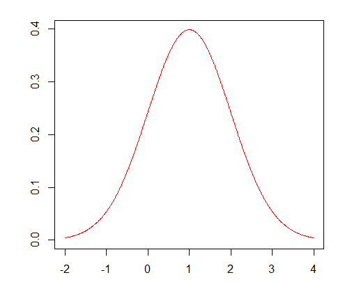
Don’t worry too much about what this graph means - basically the place where the curve is high corresponds to the more likely outcomes. In fact, it’s a normal distribution, and is really common in statistics as a way of modelling data. The key thing to notice is that the curve is symmetric, and peaks at the value 1, so “on average” we’ll earn 1 pound per day, and day-by-day our fortune will tend to grow like a straight line. That’s great! I can even check this intuition by simulating some data according to this distribution:

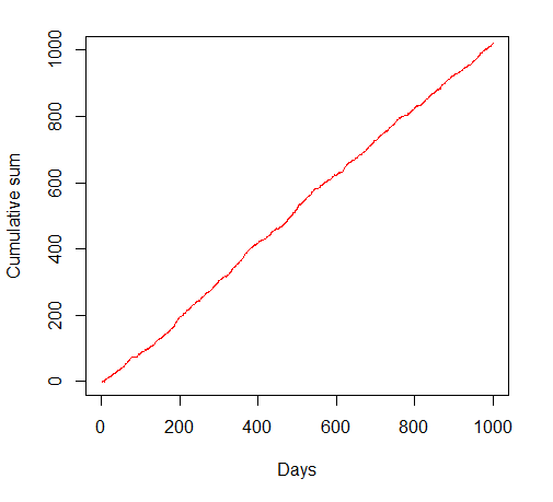
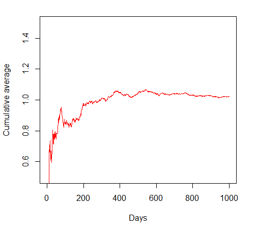
In fact, instead of looking at the cumulative sum, we can look at the cumulative average daily return. You can see that in this case, after a disappointing start the long-term average settles down to a level close to 1, as we’d expect. We are essentially guaranteed linear growth in our fortune (or, if we were bolder and used our previous winnings to boost our stake, even exponential growth).

This isn’t a surprise to mathematicians. One of the really nice things about these normal distributions is that the average of this kind of data also has a normal distribution. In fact, it comes from the same sort of bell-shaped curve, again peaked at 1, but with a much narrower and tighter peak. The range of values we might tend to see is smaller, and so we can be confident that the long-run average will be very close to 1.

It’s even better than that. A result called the Central Limit Theorem tells us that even if our data itself doesn’t come from a bell-shaped normal curve, then averages of big enough samples tend to look normal. It feels like the problem is solved: if we have an advantage in the gambling game, by appealing to the Central Limit Theorem, we can be confident we’ll come out ahead in the long run.

Except.

The difference between rigorous mathematical writing and blogging is that it’s very easy to sweep things under the carpet here. Often, that’s good. Not everyone wants to wade through a load of technical details, and it’s enough to understand the general principle. But sometimes you need to be careful.

The thing about the Central Limit Theorem is that it comes with conditions. It doesn’t say that averages of all samples tend to look normal, but rather it describes a very big family of samples for which this is true. And that’s great, but it means we have to be careful because there are natural-looking distributions which aren’t in this family and for which the Central Limit Theorem does not apply.

Take the Cauchy distribution¹. It’s named after the 19th Century Frenchman Augustin-Louis Cauchy, whose Wikipedia page is a wild ride. He was enough of a mathematical and scientific genius to be one of the 72 names inscribed on the Eiffel Tower, but was also a difficult character “moved by a deep hatred of the liberals who were taking power” and “a notoriously bad lecturer, assuming levels of understanding that only a few of his best students could reach”.

Anyway, we can compare Cauchy’s distribution (in blue) with the normal curve (in red). They don’t really look very different. They are both symmetric and peak at 1, but the key is that the Cauchy curve doesn’t drop off as fast in either direction as the normal. This means that more extreme values are more likely than for the normal. We’d say that the Cauchy distribution has heavy tails, which puts it outside the family where the Central Limit Theorem holds.

But honestly, the two curves don’t look so different do they? It’s hard to imagine that a gambling game which pays out according to the Cauchy distribution would be very different to one paying out according to the normal. And yet, if I simulate the returns, I see something very different:

I have to extend the y-axis to capture it all, but compared with our staid and predictable normal average, the Cauchy distribution (rather like its creator) makes some wild jumps. The average doesn’t seem to settle down at all. In fact, the huge downward jump after about 2 years takes us into very negative territory, wipes out all the gains so far, and could well bankrupt us (depending on what bankroll we started with). The heavy tails mean that there’s always a small but not negligible chance of very bad (or very good!) outcomes happening.

In fact, there are more pathological possibilities than just the Cauchy distribution. As I said, the average of normal data has a more tightly focused normal distribution. Curiously, the average of Cauchy data has exactly the same distribution as the original data points, which explains the fact that the average seems to wander all over the place on the graph. But there are more extreme distributions still, where the average gets more spread out over time. All of a sudden our intuition is on very shaky ground.

This may seem like mathematical nit-picking for the sake of it². However, the original and most basic mathematical model of finance, due to Bachelier in 1900, was based around market gains which follow normal distribution (Central Limit Theorem type) behaviour. This assumption underpins the classic and Nobel-winning Black-Scholes formula of 1973.

And yet, as long ago as 1963 there was evidence in the work of Mandelbrot (yes, that one) and Fama that the tails of real financial data might be heavy, that wilder fluctuations were possible than the standard theory would suggest.

Of course, people who trade financial products for a living are aware of this, and try to adapt their methods accordingly. However, these heavy tailed distributions can be a pitfall for enthusiastic amateurs who have developed their own systems. As well as traditional “win or lose” betting where the upside and downside are limited and known in advance, the development of spread betting on sports offers the potential for large gains or losses when extreme outcomes occur, potentially pushing us into the territory of heavy tailed distributions.

Since in practice we don’t ever see the curve that is generating our payoffs, it’s not immediately obvious whether it looks like the red or the blue one. It’s a subtle distinction because these two curves look very similar, and it’s possible that people only find out too late that they are gambling in a heavy-tailed scenario when they are suddenly wiped out after a long run of success.

But in general, it’s definitely worth being aware of these distinctions between light and heavy tailed distributions when dealing with risk in everyday life. By buying insurance, we seek to flatten the tails and reduce the chance of very bad outcomes (even if most of the time we never claim), and we should think about pandemic planning or earthquake-proof buildings in the same way.

This sort of mathematical language and thinking is definitely a helpful tool for trying to capture risk, and I encourage you to bring it to your everyday life.

1. Physicists call it the Lorentz distribution, but we don’t have to listen to them.

2. Heaven forbid